CS5446 8. Value function approximation
Notes for CS5446 Reinforcement Learning.
Example
之前介绍的情况都要求我们通过一个表格来进行求解, 不论是 q-value 还是 v-value. 对于 q-value 它是一个二维表格, 对于 v-value, 它是一个一维的向量.
那如果状态空间非常大, 或者连续呢, 我们怎么做? 用 value function approximation 来表示状态值来做近似(approximation). 整体的算法思路是:
对于 s 的 $v_\pi(s)$ 来说, 对它做线性拟合
$$ \hat{v}(s, w) = as + b = \phi^{T}(s)w $$- $\phi(s)$ 是 s 的特征函数, 在矩阵里是特征向量. $T$ 表示在矩阵中它是转置.
- $s$ 是状态
- $w$ 是参数, 在矩阵里是参数向量
- $\hat{v}(s, w)$
是价值函数的近似
- 对 s 来说是一种线性关系, 但是如果对 s 我们不做线形拟合, 那它可能是一种非线形关系.
- 对 w 来说是一种线性关系, 但是它永远对 w 成线性关系. 非线形的部分被 $\phi(s)$ 所吸收.
Value function approximation
正式地定义 value function approximation: 我们希望得到 $v_{\pi}(s)$ 的近似, 即 $\hat{v}(s, w)$ . 即我们希望找到一个 $w$ 使得 $\hat{v}(s, w)$ 尽可能接近 $v_{\pi}(s)$ . 那么我们可以定义如下的目标函数:
$$ J(w) = \mathbb{E}[(v_{\pi}(S) - \hat{v}(S, w))^2] $$我们的优化目标是是,希望找到一个 $w$ 使得 $J(w)$ 尽可能小. 因此我们可以用梯度下降的方式求解:
$$ \begin{aligned} & \nabla_w J(w) = \nabla \mathbb{E}[(v_{\pi}(S) - \hat{v}(S, w))^2] \\ & = \mathbb{E}[\nabla (v_{\pi}(S) - \hat{v}(S, w))^2] \\ & = 2\mathbb{E}[(v_{\pi}(S) - \hat{v}(S, w)) (- \nabla \hat{v}(S, w))] \\ & = -2\mathbb{E}[(v_{\pi}(S) - \hat{v}(S, w)) \nabla \hat{v}(S, w)] \end{aligned} $$对此我们可以用迭代的方法进行求解:
$$ \begin{aligned} & w_{t+1} = w_t - \alpha_t \nabla_w J(w_t) \\ & = w_t \red{+} \alpha_t [(v_{\pi}(s_t) - \hat{v}(s_t, w_t)) \nabla \hat{v}(s_t, w_t)] \end{aligned} $$注意上面梯度下降的式子是负的
但是这里有一个未知的值: $v_{\pi}(s_t)$ . 因此我们可以用一个估计值来代替 $v_{\pi}(s_t)$ . 我们可以通过 MC learning 或者 TD learning 的方法来估计它, 比如使用 TD learning 的方式:
$$ \begin{aligned} & w_{t+1} = w_t + \alpha_t [(v_{\pi}(s_t) - \hat{v}(s_t, w_t)) \nabla \hat{v}(s_t, w_t)] \\ & = w_t + \alpha_t [r_t + \gamma \hat{v}(s_{t+1}, w_t)- \hat{v}(s_t, w_t)] \nabla \hat{v}(s_t, w_t) \end{aligned} $$这样我们就可以用迭代法来求了:
- 我们对 $(s_t, r_t, s_{t+1})$ 进行采样
- 然后不断迭代求解 $w$ 使得 $\hat{v}(s, w)$ 最终接近 $v_{\pi}(s)$
这个算法最终解决了如何估计 state value 的问题.
$\hat{v}(s, w)$ 的选取
上面的式子中, 我们发现我们仍然需要知道 $\hat{v}(s, w)$ 的值. 因此选取拟合的方式很重要. 我们除了使用线形的方式进行拟合, 还可以通过神经网络的方式进行拟合. 神经网络本质上就是对非线形关系进行拟合.
Example: Linear Approximation
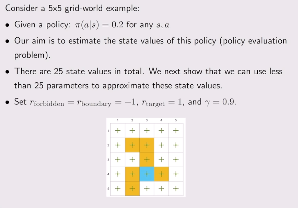
以这个例子为例, 由于这个例子的 model 我们都知道, 因此我们可以直接线形求解:
import numpy as np

H, W = 5, 5
gamma = 0.9

ACTIONS = {
    0: (-1, 0),  # up
    1: (1, 0),  # down
    2: (0, -1),  # left
    3: (0, 1),  # right
    4: (0, 0),  # stay
}
pi = 1.0 / len(ACTIONS)  # 0.2

# 1-based coordinates
forbidden = {(2, 2), (2, 3), (3, 3), (4, 2), (4, 4), (5, 2)}
target = (4, 3)

r_forbidden = -1.0
r_boundary = -1.0
r_target = 1.0


def idx(r, c):  # r,c are 1-based
    return (r - 1) * W + (c - 1)


def step(r, c, a):
    # direction row, column
    dr, dc = ACTIONS[a]
    # next row, column
    nr, nc = r + dr, c + dc

    # boundary -> stay (and get boundary reward)
    if nr < 1 or nr > H or nc < 1 or nc > W:
        return (r, c), r_boundary

    ns = (nr, nc)

    # reward by landing cell
    if ns == target:
        return ns, r_target
    if ns in forbidden:
        return ns, r_forbidden

    return ns, 0.0  # normal cell reward


S = H * W
# state transition probability matrix
P_pi = np.zeros((S, S), dtype=float)
# state reward vector
r_pi = np.zeros(S, dtype=float)

for r in range(1, H + 1):
    for c in range(1, W + 1):
        s = idx(r, c)
        for a in ACTIONS:
            (nr, nc), reward = step(r, c, a)
            sp = idx(nr, nc)
            P_pi[s, sp] += pi
            r_pi[s] += pi * reward

I = np.eye(S)
A = I - gamma * P_pi
# Solve (I - gamma P) v = r
v = np.linalg.solve(A, r_pi)
# print as 5x5
V = v.reshape(H, W)
np.set_printoptions(precision=3, suppress=True)
print("\n=== V (5x5) ===")
print(V)
注意这里的计算都是矩阵计算
np.linalg.solve(A, b)是 NumPy 里用来解线性方程组的函数:它直接求出满足 $Ax = b$ 的 $x$ 的值. 因此原先 $v = r_{\pi} + \gamma P_{\pi}v$ 被移项成了: $(I - \gamma P_{\pi})v = r_{\pi}$我们只需要构造出来 $A$ 和 $r_{\pi}$ 就可以求解出 $v$ 的值.
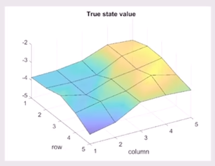
最终我们得到:
=== V (5x5) ===
[[-3.846 -3.814 -3.644 -3.121 -3.235]
 [-3.794 -3.847 -3.8   -3.106 -2.924]
 [-3.572 -3.896 -3.382 -3.194 -2.944]
 [-3.901 -3.616 -3.403 -2.898 -3.239]
 [-4.459 -4.161 -3.386 -3.363 -3.453]]
使用一个三维图像进行可视化:
有了这个答案我们可以看看如果我们用 linear approximation 来求解会怎么样.
import matplotlib.pyplot as plt
import numpy as np
from mpl_toolkits.mplot3d import Axes3D  # noqa: F401

# =========================
# 1) Gridworld definition (keep yours)
# =========================
H, W = 5, 5
gamma = 0.9

ACTIONS = {
    0: (-1, 0),  # up
    1: (1, 0),  # down
    2: (0, -1),  # left
    3: (0, 1),  # right
    4: (0, 0),  # stay
}
A = len(ACTIONS)

r_forbidden = -1.0
r_boundary = -1.0
r_target = 1.0

FORBIDDEN = {(2, 2), (2, 3), (3, 3), (4, 2), (4, 4), (5, 2)}
TARGET = (4, 3)


def step(state_rc, action):
    r, c = state_rc
    dr, dc = ACTIONS[action]
    nr, nc = r + dr, c + dc

    if nr < 1 or nr > H or nc < 1 or nc > W:
        return (r, c), r_boundary

    ns = (nr, nc)
    if ns == TARGET:
        return ns, r_target
    if ns in FORBIDDEN:
        return ns, r_forbidden
    return ns, 0.0


# =========================================
# 2) Polynomial features phi(s) up to degree K
# =========================================
def make_poly_phi(degree: int):
    """
    Build polynomial features in (rn, cn) up to total degree=degree.
    Example:
      degree=1 -> [1, rn, cn]
      degree=2 -> [1, rn, cn, rn^2, rn*cn, cn^2]
      degree=3 -> add rn^3, rn^2*cn, rn*cn^2, cn^3
    """
    assert degree >= 0

    def phi(state_rc):
        r, c = state_rc
        rn = (r - 1) / (H - 1)  # [0,1]
        cn = (c - 1) / (W - 1)  # [0,1]

        feats = [1.0]
        # total degree d: rn^i * cn^j with i+j=d
        for d in range(1, degree + 1):
            for i in range(d, -1, -1):
                j = d - i
                feats.append((rn**i) * (cn**j))
        return np.asarray(feats, dtype=np.float64)

    # feature dimension
    dim = 1 + sum((d + 1) for d in range(1, degree + 1))  # 1 + (2+3+...+degree+1)
    return phi, dim


def v_hat(state_rc, w, phi_fn):
    return float(np.dot(w, phi_fn(state_rc)))


# =========================================
# 3) TD(0) trainer
# =========================================
rng = np.random.default_rng(0)

num_episodes = 500
steps_per_episode = 500
alpha0 = 0.1


def alpha(t):
    return alpha0 / np.sqrt(1.0 + t / 2000.0)


def train_td0(phi_fn, d, seed=0):
    rng_local = np.random.default_rng(seed)
    w = np.zeros(d, dtype=np.float64)

    td_err_log = []
    t_global = 0

    for ep in range(num_episodes):
        s = (int(rng_local.integers(1, H + 1)), int(rng_local.integers(1, W + 1)))

        for _ in range(steps_per_episode):
            a = int(rng_local.integers(0, A))
            s_next, r = step(s, a)

            v_s = v_hat(s, w, phi_fn)
            v_sn = v_hat(s_next, w, phi_fn)
            delta = r + gamma * v_sn - v_s

            w += alpha(t_global) * delta * phi_fn(s)

            if t_global % 1000 == 0:
                td_err_log.append(abs(delta))

            s = s_next
            t_global += 1

    return w, np.asarray(td_err_log, dtype=np.float64)


def compute_V(w, phi_fn):
    V = np.zeros((H, W), dtype=np.float64)
    for r in range(1, H + 1):
        for c in range(1, W + 1):
            V[r - 1, c - 1] = v_hat((r, c), w, phi_fn)
    return V


# =========================================
# 4) Train for degree 1/2/3, compute V
# =========================================
degrees = [1, 2, 3]
results = {}

for deg in degrees:
    phi_fn, d = make_poly_phi(deg)
    w, td_err = train_td0(phi_fn, d, seed=0)
    V = compute_V(w, phi_fn)
    results[deg] = {"phi": phi_fn, "d": d, "w": w, "V": V, "td_err": td_err}

    print(f"\n=== degree={deg} ===")
    print("d =", d)
    print("w =", w)
    print("Estimated V =\n", np.round(V, 3))


# =========================================
# 5) 3D visualization with gradient color + colorbar
# =========================================
rows = np.arange(1, H + 1)
cols = np.arange(1, W + 1)
C, R = np.meshgrid(cols, rows)  # X=col, Y=row

# optional: use same color scale across degrees for easy comparison
all_vals = np.concatenate([results[d]["V"].ravel() for d in degrees])
vmin, vmax = float(all_vals.min()), float(all_vals.max())

for deg in degrees:
    Z = results[deg]["V"]

    fig = plt.figure(figsize=(9, 6))
    ax = fig.add_subplot(111, projection="3d")

    surf = ax.plot_surface(
        C,
        R,
        Z,
        rstride=1,
        cstride=1,
        linewidth=0,
        antialiased=True,
        cmap="viridis",  # 渐变色
        vmin=vmin,
        vmax=vmax,  # 统一色阶(想各自自适应就删掉这行)
    )

    # colorbar(显示渐变对应的数值)
    fig.colorbar(surf, ax=ax, shrink=0.7, pad=0.1, label="v_hat")

    ax.set_xlabel("col")
    ax.set_ylabel("row")
    ax.set_zlabel("v_hat(row,col)")
    ax.set_title(f"TD(0) + Poly Features (degree={deg})")
    ax.set_box_aspect((1.0, 1.0, 0.5))
    ax.invert_yaxis()
    ax.view_init(elev=30, azim=225)

    plt.savefig(f"value_surface_deg{deg}.png", dpi=300, bbox_inches="tight")
    plt.show()
我们可以看到以下结果:


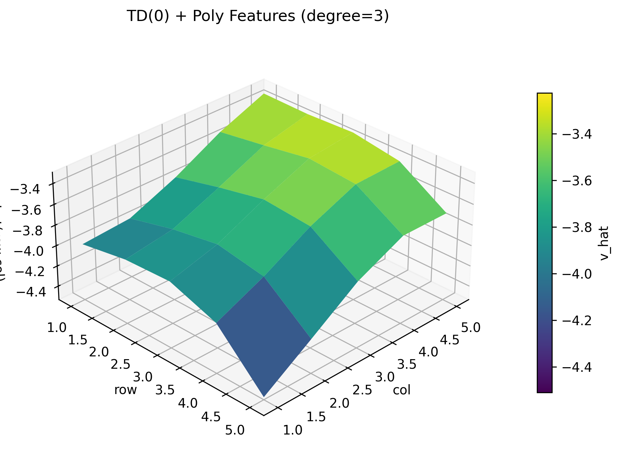
我们可以看到, 随着 degree 的增加, 拟合的效果在变好.
一句感叹… AI 好强. 这种POC的代码都不用手写了.